Classical Neural Network Module¶

The following classical neural network modules support automatic back propagation computation.After running the forward function, you can calculate the gradient by executing the reverse function.A simple example of the convolution layer is as follows:

from pyvqnet.tensor import QTensor
from pyvqnet.nn import Conv2D
from pyvqnet._core import Tensor as CoreTensor
# an image feed into two dimension convolution layer
b = 2        # batch size
ic = 2       # input channels
oc = 2      # output channels
hw = 4      # input width and heights

# two dimension convolution layer
test_conv = Conv2D(ic,oc,(2,2),(2,2),"same")

# input of shape [b,ic,hw,hw]
x0 = QTensor(CoreTensor.range(1,b*ic*hw*hw).reshape([b,ic,hw,hw]),requires_grad=True)

#forward function
x = test_conv(x0)

#backward function with autograd
x.backward()
print(x0.grad)

# [
# [[[0.3051388, 0.3040530, 0.3051388, 0.1224213],
#  [0.1118232, 0.1448178, 0.1118232, 0.2228756],
#  [0.3051388, 0.3040530, 0.3051388, 0.1224213],
#  [0.0281369, 0.2619222, 0.0281369, 0.0893420]],
# [[-0.2651831, 0.4174044, -0.2651831, 0.2255079],
#  [-0.3505684, 0.0706428, -0.3505684, 0.1537349],
#  [-0.2651831, 0.4174044, -0.2651831, 0.2255079],
#  [-0.0199047, -0.1207576, -0.0199047, 0.0083465]]],
# [[[0.3051388, 0.3040530, 0.3051388, 0.1224213],
#  [0.1118232, 0.1448178, 0.1118232, 0.2228756],
#  [0.3051388, 0.3040530, 0.3051388, 0.1224213],
#  [0.0281369, 0.2619222, 0.0281369, 0.0893420]],
# [[-0.2651831, 0.4174044, -0.2651831, 0.2255079],
#  [-0.3505684, 0.0706428, -0.3505684, 0.1537349],
#  [-0.2651831, 0.4174044, -0.2651831, 0.2255079],
#  [-0.0199047, -0.1207576, -0.0199047, 0.0083465]]]
# ]

Module Class¶

abstract calculation module

Module¶

class pyvqnet.nn.module.Module¶

Base class for all neural network modules including quantum modules or classic modules. Your models should also be subclass of this class for autograd calculation.

Modules can also contain other Modules, allowing to nest them in a tree structure. You can assign the submodules as regular attributes:

class Model(Module):
    def __init__(self):
        super(Model, self).__init__()
        self.conv1 = pyvqnet.nn.Conv2d(1, 20, (5,5))
        self.conv2 = pyvqnet.nn.Conv2d(20, 20, (5,5))

    def forward(self, x):
        x = pyvqnet.nn.activation.relu(self.conv1(x))
        return pyvqnet.nn.activation.relu(self.conv2(x))

Submodules assigned in this way will be registered

forward¶

pyvqnet.nn.module.Module.forward(x, *args, **kwargs)¶

Abstract method which performs forward pass.

Parameters

x – input QTensor
*args – A non-keyword variable parameter
**kwargs – A keyword variable parameter

Returns

module output

Example:

import numpy as np
from pyvqnet.tensor import QTensor
from pyvqnet.nn import Conv2D
b= 2
ic = 3
oc = 2
test_conv = Conv2D(ic,oc,(3,3),(2,2),"same")
x0 = QTensor(np.arange(1,b*ic*5*5+1).reshape([b,ic,5,5]),requires_grad=True)
x = test_conv.forward(x0)
print(x)

# [
# [[[4.3995643, 3.9317808, -2.0707254],
#  [20.1951981, 21.6946659, 14.2591858],
#  [38.4702759, 31.9730244, 24.5977650]],
# [[-17.0607567, -31.5377998, -7.5618000],
#  [-22.5664024, -40.3876266, -15.1564388],
#  [-3.1080279, -18.5986233, -8.0648050]]],
# [[[6.6493244, -13.4840755, -20.2554188],
#  [54.4235802, 34.4462433, 26.8171902],
#  [90.2827682, 62.9092331, 51.6892929]],
# [[-22.3385429, -45.2448578, 5.7101378],
#  [-32.9464149, -60.9557228, -10.4994345],
#  [5.9029331, -20.5480480, -0.9379558]]]
# ]

state_dict¶

pyvqnet.nn.module.Module.state_dict(destination=None, prefix='')¶

Return a dictionary containing a whole state of the module.

Both parameters and persistent buffers (e.g. running averages) are included. Keys are corresponding parameter and buffer names.

Parameters

destination – a dict where state will be stored
prefix – the prefix for parameters and buffers used in this module

Returns

a dictionary containing a whole state of the module

Example:

from pyvqnet.nn import Conv2D
test_conv = Conv2D(2,3,(3,3),(2,2),"same")
print(test_conv.state_dict().keys())
#odict_keys(['weights', 'bias'])

save_parameters¶

pyvqnet.utils.storage.save_parameters(obj, f)¶

Saves model parmeters to a disk file.

Parameters

obj – saved OrderedDict from state_dict()
f – a string or os.PathLike object containing a file name

Returns

None

Example:

from pyvqnet.nn import Module,Conv2D
import pyvqnet
class Net(Module):
    def __init__(self):
        super(Net, self).__init__()
        self.conv1 = Conv2D(input_channels=1, output_channels=6, kernel_size=(5, 5), stride=(1, 1), padding="valid")

    def forward(self, x):
        return super().forward(x)

model = Net()
pyvqnet.utils.storage.save_parameters(model.state_dict(),"tmp.model")

load_parameters¶

pyvqnet.utils.storage.load_parameters(f)¶

Loads model paramters from a disk file.

The model instance should be created first.

Parameters: f – a string or os.PathLike object containing a file name
Returns: saved OrderedDict for load_state_dict()

Example:

from pyvqnet.nn import Module,Conv2D
import pyvqnet

class Net(Module):
    def __init__(self):
        super(Net, self).__init__()
        self.conv1 = Conv2D(input_channels=1, output_channels=6, kernel_size=(5, 5), stride=(1, 1), padding="valid")

    def forward(self, x):
        return super().forward(x)

model = Net()
model1 = Net()  # another Module object
pyvqnet.utils.storage.save_parameters( model.state_dict(),"tmp.model")
model_para =  pyvqnet.utils.storage.load_parameters("tmp.model")
model1.load_state_dict(model_para)

Classical Neural Network Layer¶

Conv1D¶

class pyvqnet.nn.Conv1D(input_channels: int, output_channels: int, kernel_size: int, stride: int = 1, padding='valid', use_bias: str = True, kernel_initializer=None, bias_initializer=None, dilation_rate: int = 1, group: int = 1)¶

Apply a 1-dimensional convolution kernel over an input . Inputs to the conv module are of shape (batch_size, input_channels, height)

Parameters

input_channels – int - Number of input channels
output_channels – int - Number of kernels
kernel_size – int - Size of a single kernel. kernel shape = [output_channels,input_channels/group,kernel_size,1]
stride – int - Stride, defaults to 1
padding – str|int - padding option, which can be a string {‘valid’, ‘same’} or an integer giving the amount of implicit padding to apply . Default “valid”.
use_bias – bool - if use bias, defaults to True
kernel_initializer – callable - Defaults to None
bias_initializer – callable - Defaults to None
dilation_rate – int - dilated size, defaults: 1
group – int - number of groups of grouped convolutions. Default: 1

Returns

a Conv1D class

Note

padding='valid' is the same as no padding.

padding='same' pads the input so the output has the shape as the input.

Example:

import numpy as np
from pyvqnet.tensor import QTensor
from pyvqnet.nn import Conv1D
b= 2
ic =3
oc = 2
test_conv = Conv1D(ic,oc,3,2,"same")
x0 = QTensor(np.arange(1,b*ic*5*5 +1).reshape([b,ic,25]),requires_grad=True)
x = test_conv.forward(x0)
print(x)

# [
# [[12.4438553, 14.8618164, 15.5595102, 16.2572021, 16.9548950, 17.6525879, 18.3502808, 19.0479736, 19.7456665, 20.4433594, 21.1410522, 21.8387432, 10.5725441],
#  [-13.7539215, 1.0263026, 1.2747254, 1.5231485, 1.7715728, 2.0199962, 2.2684195, 2.5168428, 2.7652662, 3.0136888, 3.2621140, 3.5105357, 14.0515862]],
# [[47.4924164, 41.0252953, 41.7229881, 42.4206772, 43.1183739, 43.8160667, 44.5137596, 45.2114487, 45.9091415, 46.6068344, 47.3045311, 48.0022240, 18.3216572],
#  [-47.2381554, 10.3421783, 10.5906038, 10.8390274, 11.0874519, 11.3358765, 11.5842953, 11.8327246, 12.0811434, 12.3295631, 12.5779924, 12.8264122, 39.4719162]]
# ]

Conv2D¶

class pyvqnet.nn.Conv2D(input_channels: int, output_channels: int, kernel_size: tuple, stride: tuple = (1, 1), padding='valid', use_bias=True, kernel_initializer=None, bias_initializer=None, dilation_rate: int = 1, group: int = 1)¶

Apply a two-dimensional convolution kernel over an input . Inputs to the conv module are of shape (batch_size, input_channels, height, width)

Parameters

input_channels – int - Number of input channels
output_channels – int - Number of kernels
kernel_size – tuple|list - Size of a single kernel. kernel shape = [output_channels,input_channels/group,kernel_size,kernel_size]
stride – tuple|list - Stride, defaults to (1, 1)|[1,1]
padding – str|tuple - padding option, which can be a string {‘valid’, ‘same’} or a tuple of integers giving the amount of implicit padding to apply on both sides. Default “valid”.
use_bias – bool - if use bias, defaults to True
kernel_initializer – callable - Defaults to None
bias_initializer – callable - Defaults to None
dilation_rate – int - dilated size, defaults: 1
group – int - number of groups of grouped convolutions. Default: 1

Returns

a Conv2D class

Note

padding='valid' is the same as no padding.

padding='same' pads the input so the output has the shape as the input.

Example:

import numpy as np
from pyvqnet.tensor import QTensor
from pyvqnet.nn import Conv2D
b= 2
ic =3
oc = 2
test_conv = Conv2D(ic,oc,(3,3),(2,2),"same")
x0 = QTensor(np.arange(1,b*ic*5*5+1).reshape([b,ic,5,5]),requires_grad=True)
x = test_conv.forward(x0)
print(x)

# [
# [[[-0.1256833, 23.8978596, 26.7449780],
#  [-7.2959919, 33.4023743, 42.1283913],
#  [-8.7684336, 25.2698975, 40.4024887]],
# [[33.0653763, 40.3120155, 27.3781891],
#  [39.2921371, 45.8685760, 38.1885109],
#  [23.1873779, 12.0480318, 12.7278290]]],
# [[[-0.9730744, 61.3967094, 79.0511856],
#  [-29.3652401, 75.0349350, 112.7325439],
#  [-26.4682808, 59.0924797, 104.2572098]],
# [[66.8064194, 96.0953140, 72.9157486],
#  [90.9154129, 110.7232437, 91.2616043],
#  [56.8825951, 34.6904907, 30.1957760]]]
# ]

ConvT2D¶

class pyvqnet.nn.ConvT2D(input_channels, output_channels, kernel_size, stride=[1, 1], padding='valid', use_bias='True', kernel_initializer=None, bias_initializer=None, dilation_rate: int = 1, group: int = 1)¶

Apply a two-dimensional transposed convolution kernel over an input. Inputs to the convT module are of shape (batch_size, input_channels, height, width)

Parameters

input_channels – int - Number of input channels
output_channels – int - Number of kernels
kernel_size – tuple|list - Size of a single kernel. kernel shape = [input_channels,output_channels/group,kernel_size,kernel_size]
stride – tuple|list - Stride, defaults to (1, 1)|[1,1]
padding – str|tuple - padding option, which can be a string {‘valid’, ‘same’} or a tuple of integers giving the amount of implicit padding to apply on both sides. Default “valid”.
use_bias – bool - Whether to use a offset item. Default to use
kernel_initializer – callable - Defaults to None
bias_initializer – callable - Defaults to None
dilation_rate – int - dilated size, defaults: 1
group – int - number of groups of grouped convolutions. Default: 1

Returns

a ConvT2D class

Note

padding='valid' is the same as no padding.

padding='same' pads the input so the output has the shape as the input.

Example:

import numpy as np
from pyvqnet.tensor import QTensor
from pyvqnet.nn import ConvT2D
test_conv = ConvT2D(3, 2, (3, 3), (1, 1), "valid")
x = QTensor(np.arange(1, 1 * 3 * 5 * 5+1).reshape([1, 3, 5, 5]), requires_grad=True)
y = test_conv.forward(x)
print(y)

# [
# [[[-3.3675897, 4.8476148, 14.2448473, 14.8897810, 15.5347166, 20.0420666, 10.9831696],
#  [-14.0110836, -3.2500827, 6.4022207, 6.5149083, 6.6275964, 23.7946320, 12.1828709],
#  [-22.2661152, -3.5112300, 12.9493723, 13.5486069, 14.1478367, 39.6327629, 18.8349991],
#  [-24.4063797, -3.0093837, 15.9455290, 16.5447617, 17.1439915, 44.7691879, 21.3293095],
#  [-26.5466480, -2.5075383, 18.9416828, 19.5409145, 20.1401463, 49.9056053, 23.8236179],
#  [-24.7624626, -13.7395811, -7.9510674, -7.9967723, -8.0424776, 19.2783546, 7.0562835],
#  [-3.5170188, 10.2280807, 16.1939259, 16.6804695, 17.1670132, 21.2262039, 6.2889833]],
# [[-2.0570512, -9.5056667, -25.0429192, -25.9464111, -26.8499031, -24.7305946, -16.9881954],
#  [-0.7620960, -18.3383904, -49.8948288, -51.2528229, -52.6108208, -52.2179604, -34.3664169],
#  [-11.7121849, -27.1864738, -62.2154846, -63.6433640, -65.0712280, -52.6787071, -38.4497032],
#  [-13.3643141, -29.0211792, -69.3548126, -70.7826691, -72.2105408, -58.1659012, -43.7543182],
#  [-15.0164423, -30.8558884, -76.4941254, -77.9219971, -79.3498535, -63.6530838, -49.0589256],
#  [-11.6070204, -14.1940546, -35.5471687, -36.0715408, -36.5959129, -23.9147663, -22.8668022],
#  [-14.4390459, -4.9011412, -6.4719801, -6.5418491, -6.6117167, 9.3329525, -1.7254852]]]
# ]

AvgPool1D¶

class pyvqnet.nn.AvgPool1D(kernel, stride, padding='valid', name='')¶

This operation applies a 1D average pooling over an input signal composed of several input planes.

Parameters

kernel – size of the average pooling windows
strides – factor by which to downscale
padding – one of “valid”, “same” or integer specifies the padding value, defaults to “valid”
name – name of the output layer

Returns

AvgPool1D layer

Note

padding='valid' is the same as no padding.

padding='same' pads the input so the output has the shape as the input.

Example:

import numpy as np
from pyvqnet.tensor import QTensor
from pyvqnet.nn import AvgPool1D
test_mp = AvgPool1D([3],[2],"same")
x= QTensor(np.array([0, 1, 0, 4, 5,
                            2, 3, 2, 1, 3,
                            4, 4, 0, 4, 3,
                            2, 5, 2, 6, 4,
                            1, 0, 0, 5, 7],dtype=float).reshape([1,5,5]),requires_grad=True)

y= test_mp.forward(x)
print(y)

# [
# [[0.3333333, 1.6666666, 3.0000000],
#  [1.6666666, 2.0000000, 1.3333334],
#  [2.6666667, 2.6666667, 2.3333333],
#  [2.3333333, 4.3333335, 3.3333333],
#  [0.3333333, 1.6666666, 4.0000000]]
# ]

MaxPool1D¶

class pyvqnet.nn.MaxPool1D(kernel, stride, padding='valid', name='')¶

This operation applies a 1D max pooling over an input signal composed of several input planes.

Parameters

kernel – size of the max pooling windows
strides – factor by which to downscale
padding – one of “valid”, “same” or integer specifies the padding value, defaults to “valid”
name – name of the output layer

Returns

MaxPool1D layer

Note

padding='valid' is the same as no padding.

padding='same' pads the input so the output has the shape as the input.

Example:

import numpy as np
from pyvqnet.tensor import QTensor
from pyvqnet.nn import MaxPool1D
test_mp = MaxPool1D([3],[2],"same")
x= QTensor(np.array([0, 1, 0, 4, 5,
                            2, 3, 2, 1, 3,
                            4, 4, 0, 4, 3,
                            2, 5, 2, 6, 4,
                            1, 0, 0, 5, 7],dtype=float).reshape([1,5,5]),requires_grad=True)

y= test_mp.forward(x)
print(y)
# [
# [[1.0000000, 4.0000000, 5.0000000],
#  [3.0000000, 3.0000000, 3.0000000],
#  [4.0000000, 4.0000000, 4.0000000],
#  [5.0000000, 6.0000000, 6.0000000],
#  [1.0000000, 5.0000000, 7.0000000]]
# ]

AvgPool2D¶

class pyvqnet.nn.AvgPool2D(kernel, stride, padding='valid', name='')¶

This operation applies 2D average pooling over input features .

Parameters

kernel – size of the average pooling windows
strides – factors by which to downscale
padding – one of “valid”, “same” or tuple with integers specifies the padding value of column and row,defaults to “valid”
name – name of the output layer

Returns

AvgPool2D layer

Note

padding='valid' is the same as no padding.

padding='same' pads the input so the output has the shape as the input.

Example:

import numpy as np
from pyvqnet.tensor import QTensor
from pyvqnet.nn import AvgPool2D
test_mp = AvgPool2D([2,2],[2,2],"valid")
x= QTensor(np.array([0, 1, 0, 4, 5,
                            2, 3, 2, 1, 3,
                            4, 4, 0, 4, 3,
                            2, 5, 2, 6, 4,
                            1, 0, 0, 5, 7],dtype=float).reshape([1,1,5,5]),requires_grad=True)

y= test_mp.forward(x)
print(y)
# [
# [[[1.5000000, 1.7500000],
#  [3.7500000, 3.0000000]]]
# ]

MaxPool2D¶

class pyvqnet.nn.MaxPool2D(kernel, stride, padding='valid', name='')¶

This operation applies 2D max pooling over input features.

Parameters

kernel – size of the max pooling windows
strides – factor by which to downscale
padding – one of “valid”, “same” or tuple with integers specifies the padding value of column and row, defaults to “valid”
name – name of the output layer

Returns

MaxPool2D layer

Note

padding='valid' is the same as no padding.

padding='same' pads the input so the output has the shape as the input.

Example:

import numpy as np
from pyvqnet.tensor import QTensor
from pyvqnet.nn import MaxPool2D
test_mp = MaxPool2D([2,2],[2,2],"valid")
x= QTensor(np.array([0, 1, 0, 4, 5,
                            2, 3, 2, 1, 3,
                            4, 4, 0, 4, 3,
                            2, 5, 2, 6, 4,
                            1, 0, 0, 5, 7],dtype=float).reshape([1,1,5,5]),requires_grad=True)

y= test_mp.forward(x)
print(y)
# [
# [[[3.0000000, 4.0000000],
#  [5.0000000, 6.0000000]]]
# ]

Embedding¶

class pyvqnet.nn.embedding.Embedding(num_embeddings, embedding_dim, weight_initializer=<function xavier_normal>, name: str = '')¶

This module is often used to store word embeddings and retrieve them using indices. The input to the module is a list of indices, and the output is the corresponding word embeddings.

Parameters

num_embeddings – int - size of the dictionary of embeddings
embedding_dim – int - the size of each embedding vector
weight_initializer – callable - defaults to normal
name – name of the output layer

Returns

a Embedding class

Example:

import numpy as np
from pyvqnet.tensor import QTensor
from pyvqnet.nn.embedding import Embedding
vlayer = Embedding(30,3)
x = QTensor(np.arange(1,25).reshape([2,3,2,2]))
y = vlayer(x)
print(y)

# [
# [[[[-0.3168081, 0.0329394, -0.2934906],
#  [0.1057295, -0.2844988, -0.1687456]],
# [[-0.2382513, -0.3642318, -0.2257225],
#  [0.1563180, 0.1567665, 0.3038477]]],
# [[[-0.4131152, -0.0564500, -0.2804018],
#  [-0.2955172, -0.0009581, -0.1641144]],
# [[0.0692555, 0.1094901, 0.4099118],
#  [0.4348361, 0.0304361, -0.0061203]]],
# [[[-0.3310401, -0.1836129, 0.1098949],
#  [-0.1840732, 0.0332474, -0.0261806]],
# [[-0.1489778, 0.2519453, 0.3299376],
#  [-0.1942692, -0.1540277, -0.2335350]]]],
# [[[[-0.2620637, -0.3181309, -0.1857461],
#  [-0.0878164, -0.4180320, -0.1831555]],
# [[-0.0738970, -0.1888980, -0.3034399],
#  [0.1955448, -0.0409723, 0.3023460]]],
# [[[0.2430045, 0.0880465, 0.4309453],
#  [-0.1796514, -0.1432367, -0.1253638]],
# [[-0.5266719, 0.2386262, -0.0329155],
#  [0.1033449, -0.3442690, -0.0471130]]],
# [[[-0.5336705, -0.1939755, -0.3000667],
#  [0.0059001, 0.5567381, 0.1926173]],
# [[-0.2385869, -0.3910453, 0.2521235],
#  [-0.0246447, -0.0241158, -0.1402829]]]]
# ]

BatchNorm2d¶

class pyvqnet.nn.BatchNorm2d(channel_num: int, momentum: float = 0.1, epsilon: float = 1e-05, beta_initializer=zeros, gamma_initializer=ones, name='')¶

Applies Batch Normalization over a 4D input (B,C,H,W) as described in the paper Batch Normalization: Accelerating Deep Network Training by Reducing Internal Covariate Shift .

\[y = \frac{x - \mathrm{E}[x]}{\sqrt{\mathrm{Var}[x] + \epsilon}} * \gamma + \beta\]

where \(\gamma\) and \(\beta\) are learnable parameters.Also by default, during training this layer keeps running estimates of its computed mean and variance, which are then used for normalization during evaluation. The running estimates are kept with a default momentum of 0.1.

Parameters

channel_num – int - the number of input features channels
momentum – float - momentum when calculation exponentially weighted average, defaults to 0.1
beta_initializer – callable - defaults to zeros
gamma_initializer – callable - defaults to ones
epsilon – float - numerical stability constant, defaults to 1e-5
name – name of the output layer

Returns

a BatchNorm2d class

Example:

import numpy as np
from pyvqnet.tensor import QTensor
from pyvqnet.nn import BatchNorm2d
b= 2
ic =2
test_conv = BatchNorm2d(ic)

x = QTensor(np.arange(1,17).reshape([b,ic,4,1]),requires_grad=True)
y = test_conv.forward(x)
print(y)

# [
# [[[-1.3242440],
#  [-1.0834724],
#  [-0.8427007],
#  [-0.6019291]],
# [[-1.3242440],
#  [-1.0834724],
#  [-0.8427007],
#  [-0.6019291]]],
# [[[0.6019291],
#  [0.8427007],
#  [1.0834724],
#  [1.3242440]],
# [[0.6019291],
#  [0.8427007],
#  [1.0834724],
#  [1.3242440]]]
# ]

BatchNorm1d¶

class pyvqnet.nn.BatchNorm1d(channel_num: int, momentum: float = 0.1, epsilon: float = 1e-05, beta_initializer=zeros, gamma_initializer=ones, name='')¶

Applies Batch Normalization over a 2D input (B,C) as described in the paper Batch Normalization: Accelerating Deep Network Training by Reducing Internal Covariate Shift .

\[y = \frac{x - \mathrm{E}[x]}{\sqrt{\mathrm{Var}[x] + \epsilon}} * \gamma + \beta\]

where \(\gamma\) and \(\beta\) are learnable parameters.Also by default, during training this layer keeps running estimates of its computed mean and variance, which are then used for normalization during evaluation. The running estimates are kept with a default momentum of 0.1.

Parameters

channel_num – int - the number of input features channels
momentum – float - momentum when calculation exponentially weighted average, defaults to 0.1
beta_initializer – callable - defaults to zeros
gamma_initializer – callable - defaults to ones
epsilon – float - numerical stability constant, defaults to 1e-5
name – name of the output layer

Returns

a BatchNorm1d class

Example:

import numpy as np
from pyvqnet.tensor import QTensor
from pyvqnet.nn import BatchNorm1d
test_conv = BatchNorm1d(4)

x = QTensor(np.arange(1,17).reshape([4,4]),requires_grad=True)
y = test_conv.forward(x)
print(y)

# [
# [-1.3416405, -1.3416405, -1.3416405, -1.3416405],
# [-0.4472135, -0.4472135, -0.4472135, -0.4472135],
# [0.4472135, 0.4472135, 0.4472135, 0.4472135],
# [1.3416405, 1.3416405, 1.3416405, 1.3416405]
# ]

LayerNormNd¶

class pyvqnet.nn.layer_norm.LayerNormNd(normalized_shape: list, epsilon: float = 1e-05, affine: bool = True, name='')¶

Layer normalization is performed on the last several dimensions of any input. The specific method is as described in the paper: Layer Normalization。

\[y = \frac{x - \mathrm{E}[x]}{ \sqrt{\mathrm{Var}[x] + \epsilon}} * \gamma + \beta\]

For inputs like (B,C,H,W,D), norm_shape can be [C,H,W,D],[H,W,D],[W,D] or [D] .

Parameters

norm_shape – float - standardize the shape.
epsilon – float - numerical stability constant, defaults to 1e-5.
affine – bool - whether to use the applied affine transformation, the default is True.
name – name of the output layer.

Returns

a LayerNormNd class.

Example:

import numpy as np
from pyvqnet.tensor import QTensor
from pyvqnet.nn.layer_norm import LayerNormNd
ic = 4
test_conv = LayerNormNd([2,2])
x = QTensor(np.arange(1,17).reshape([2,2,2,2]),requires_grad=True)
y = test_conv.forward(x)
print(y)
# [
# [[[-1.3416355, -0.4472118],
#  [0.4472118, 1.3416355]],
# [[-1.3416355, -0.4472118],
#  [0.4472118, 1.3416355]]],
# [[[-1.3416355, -0.4472118],
#  [0.4472118, 1.3416355]],
# [[-1.3416355, -0.4472118],
#  [0.4472118, 1.3416355]]]
# ]

LayerNorm2d¶

class pyvqnet.nn.layer_norm.LayerNorm2d(norm_size: int, epsilon: float = 1e-05, affine: bool = True, name='')¶

Applies Layer Normalization over a mini-batch of 4D inputs as described in the paper Layer Normalization

\[y = \frac{x - \mathrm{E}[x]}{ \sqrt{\mathrm{Var}[x] + \epsilon}} * \gamma + \beta\]

The mean and standard-deviation are calculated over the last D dimensions size.

For input like (B,C,H,W), norm_size should equals to C * H * W.

Parameters

norm_size – float - normalize size,equals to C * H * W
epsilon – float - numerical stability constant, defaults to 1e-5
affine – bool - whether to use the applied affine transformation, the default is True
name – name of the output layer

Returns

a LayerNorm2d class

Example:

import numpy as np
from pyvqnet.tensor import QTensor
from pyvqnet.nn.layer_norm import LayerNorm2d
ic = 4
test_conv = LayerNorm2d(8)
x = QTensor(np.arange(1,17).reshape([2,2,4,1]),requires_grad=True)
y = test_conv.forward(x)
print(y)

# [
# [[[-1.5275238],
#  [-1.0910884],
#  [-0.6546531],
#  [-0.2182177]],
# [[0.2182177],
#  [0.6546531],
#  [1.0910884],
#  [1.5275238]]],
# [[[-1.5275238],
#  [-1.0910884],
#  [-0.6546531],
#  [-0.2182177]],
# [[0.2182177],
#  [0.6546531],
#  [1.0910884],
#  [1.5275238]]]
# ]

LayerNorm1d¶

class pyvqnet.nn.layer_norm.LayerNorm1d(norm_size: int, epsilon: float = 1e-05, affine: bool = True, name='')¶

Applies Layer Normalization over a mini-batch of 2D inputs as described in the paper Layer Normalization

\[y = \frac{x - \mathrm{E}[x]}{ \sqrt{\mathrm{Var}[x] + \epsilon}} * \gamma + \beta\]

The mean and standard-deviation are calculated over the last dimensions size, where norm_size is the value of last dim size.

Parameters

norm_size – float - normalize size,equals to last dim
epsilon – float - numerical stability constant, defaults to 1e-5
affine – bool - whether to use the applied affine transformation, the default is True
name – name of the output layer

Returns

a LayerNorm1d class

Example:

import numpy as np
from pyvqnet.tensor import QTensor
from pyvqnet.nn.layer_norm import LayerNorm1d
test_conv = LayerNorm1d(4)
x = QTensor(np.arange(1,17).reshape([4,4]),requires_grad=True)
y = test_conv.forward(x)
print(y)

# [
# [-1.3416355, -0.4472118, 0.4472118, 1.3416355],
# [-1.3416355, -0.4472118, 0.4472118, 1.3416355],
# [-1.3416355, -0.4472118, 0.4472118, 1.3416355],
# [-1.3416355, -0.4472118, 0.4472118, 1.3416355]
# ]

Linear¶

class pyvqnet.nn.Linear(input_channels, output_channels, weight_initializer=None, bias_initializer=None, use_bias=True, name: str = '')¶

Linear module (fully-connected layer). \(y = Ax + b\)

Parameters

input_channels – int - number of inputs features
output_channels – int - number of output features
weight_initializer – callable - defaults to normal
bias_initializer – callable - defaults to zeros
use_bias – bool - defaults to True
name – name of the output layer

Returns

a Linear class

Example:

import numpy as np
from pyvqnet.tensor import QTensor
from pyvqnet.nn import Linear
c1 =2
c2 = 3
cin = 7
cout = 5
n = Linear(cin,cout)
input = QTensor(np.arange(1,c1*c2*cin+1).reshape((c1,c2,cin)),requires_grad=True)
y = n.forward(input)
print(y)

# [
# [[4.3084583, -1.9228780, -0.3428757, 1.2840536, -0.5865945],
#  [9.8339605, -5.5135884, -3.1228657, 4.3025794, -4.1492314],
#  [15.3594627, -9.1042995, -5.9028554, 7.3211040, -7.7118683]],
# [[20.8849659, -12.6950111, -8.6828451, 10.3396301, -11.2745066],
#  [26.4104652, -16.2857227, -11.4628344, 13.3581581, -14.8371439],
#  [31.9359703, -19.8764324, -14.2428246, 16.3766804, -18.3997803]]
# ]

Dropout¶

class pyvqnet.nn.dropout.Dropout(dropout_rate=0.5)¶

Dropout module.The dropout module randomly sets the outputs of some units to zero, while upscale others according to the given dropout probability.

Parameters: dropout_rate – float - probability that a neuron will be set to zero
Returns: a Dropout class

Example:

from pyvqnet._core import Tensor as CoreTensor
from pyvqnet.nn.dropout import Dropout
import numpy as np
from pyvqnet.tensor import QTensor
b = 2
ic = 2
x = QTensor(CoreTensor.range(-1*ic*2*2,(b-1)*ic*2*2-1).reshape([b,ic,2,2]),requires_grad=True)
droplayer = Dropout(0.5)
droplayer.train()
y = droplayer(x)
print(y)

# [
# [[[-16.0000000, -14.0000000],
#  [-0.0000000, -0.0000000]],
# [[-8.0000000, -6.0000000],
#  [-4.0000000, -2.0000000]]],
# [[[0.0000000, 2.0000000],
#  [4.0000000, 6.0000000]],
# [[8.0000000, 10.0000000],
#  [0.0000000, 14.0000000]]]
# ]

GRU¶

class pyvqnet.nn.gru.GRU(input_size, hidden_size, num_layers=1, nonlinearity='tanh', batch_first=True, use_bias=True, bidirectional=False)¶

Gated Recurrent Unit (GRU) module. Support multi-layer stacking, bidirectional configuration. The calculation formula of the single-layer one-way GRU is as follows:

\[\begin{split}\begin{array}{ll} r_t = \sigma(W_{ir} x_t + b_{ir} + W_{hr} h_{(t-1)} + b_{hr}) \\ z_t = \sigma(W_{iz} x_t + b_{iz} + W_{hz} h_{(t-1)} + b_{hz}) \\ n_t = \tanh(W_{in} x_t + b_{in} + r_t * (W_{hn} h_{(t-1)}+ b_{hn})) \\ h_t = (1 - z_t) * n_t + z_t * h_{(t-1)} \end{array}\end{split}\]

Parameters

input_size – Input feature dimensions.
hidden_size – Hidden feature dimensions.
num_layers – Stack layer numbers. default: 1.
batch_first – If batch_first is True, input shape should be [batch_size,seq_len,feature_dim], if batch_first is False, the input shape should be [seq_len,batch_size,feature_dim],default: True.
use_bias – If use_bias is False, this module will not contain bias. default: True.
bidirectional – If bidirectional is True, the module will be bidirectional GRU. default: False.

Returns

A GRU module instance.

Example:

from pyvqnet.nn import GRU
from pyvqnet.tensor import tensor

rnn2 = GRU(4, 6, 2, batch_first=False, bidirectional=True)

input = tensor.ones([5, 3, 4])
h0 = tensor.ones([4, 3, 6])

output, hn = rnn2(input, h0)
print(output)
print(hn)
# [
# [[0.2815045, 0.2056844, 0.0750246, 0.5802019, 0.3536537, 0.8136684, -0.0034523, 0.1634004, 0.6099871, 0.8451654, -0.2833570, 0.7294812],
#  [0.2815045, 0.2056844, 0.0750246, 0.5802019, 0.3536537, 0.8136684, -0.0034523, 0.1634004, 0.6099871, 0.8451654, -0.2833570, 0.7294812],
#  [0.2815045, 0.2056844, 0.0750246, 0.5802019, 0.3536537, 0.8136684, -0.0034523, 0.1634004, 0.6099871, 0.8451654, -0.2833570, 0.7294812]],
# [[0.0490867, 0.0115325, -0.2797680, 0.4711050, -0.0687061, 0.7216146, 0.0258964, 0.0619203, 0.6341010, 0.8445141, -0.4164453, 0.7409840],
#  [0.0490867, 0.0115325, -0.2797680, 0.4711050, -0.0687061, 0.7216146, 0.0258964, 0.0619203, 0.6341010, 0.8445141, -0.4164453, 0.7409840],
#  [0.0490867, 0.0115325, -0.2797680, 0.4711050, -0.0687061, 0.7216146, 0.0258964, 0.0619203, 0.6341010, 0.8445141, -0.4164453, 0.7409840]],
# [[0.0182974, -0.0536071, -0.4478674, 0.4315647, -0.2191887, 0.6492687, 0.1572548, 0.0839213, 0.6707115, 0.8444533, -0.3811499, 0.7448123],
#  [0.0182974, -0.0536071, -0.4478674, 0.4315647, -0.2191887, 0.6492687, 0.1572548, 0.0839213, 0.6707115, 0.8444533, -0.3811499, 0.7448123],
#  [0.0182974, -0.0536071, -0.4478674, 0.4315647, -0.2191887, 0.6492687, 0.1572548, 0.0839213, 0.6707115, 0.8444533, -0.3811499, 0.7448123]],
# [[0.0722285, -0.0636698, -0.5457084, 0.3817562, -0.1890205, 0.5696942, 0.3855782, 0.2057217, 0.7370453, 0.8646453, -0.1967214, 0.7630759],
#  [0.0722285, -0.0636698, -0.5457084, 0.3817562, -0.1890205, 0.5696942, 0.3855782, 0.2057217, 0.7370453, 0.8646453, -0.1967214, 0.7630759],
#  [0.0722285, -0.0636698, -0.5457084, 0.3817562, -0.1890205, 0.5696942, 0.3855782, 0.2057217, 0.7370453, 0.8646453, -0.1967214, 0.7630759]],
# [[0.1834545, -0.0489200, -0.6343678, 0.3061281, -0.0449328, 0.4901535, 0.6941375, 0.4570828, 0.8433002, 0.9152645, 0.2342478, 0.8299093],
#  [0.1834545, -0.0489200, -0.6343678, 0.3061281, -0.0449328, 0.4901535, 0.6941375, 0.4570828, 0.8433002, 0.9152645, 0.2342478, 0.8299093],
#  [0.1834545, -0.0489200, -0.6343678, 0.3061281, -0.0449328, 0.4901535, 0.6941375, 0.4570828, 0.8433002, 0.9152645, 0.2342478, 0.8299093]]
# ]
# [
# [[-0.8070476, -0.5560303, 0.7575479, -0.2368367, 0.4228620, -0.2573725],
#  [-0.8070476, -0.5560303, 0.7575479, -0.2368367, 0.4228620, -0.2573725],
#  [-0.8070476, -0.5560303, 0.7575479, -0.2368367, 0.4228620, -0.2573725]],
# [[-0.3857390, -0.3195596, 0.0281313, 0.8734715, -0.4499536, 0.2270730],
#  [-0.3857390, -0.3195596, 0.0281313, 0.8734715, -0.4499536, 0.2270730],
#  [-0.3857390, -0.3195596, 0.0281313, 0.8734715, -0.4499536, 0.2270730]],
# [[0.1834545, -0.0489200, -0.6343678, 0.3061281, -0.0449328, 0.4901535],
#  [0.1834545, -0.0489200, -0.6343678, 0.3061281, -0.0449328, 0.4901535],
#  [0.1834545, -0.0489200, -0.6343678, 0.3061281, -0.0449328, 0.4901535]],
# [[-0.0034523, 0.1634004, 0.6099871, 0.8451654, -0.2833570, 0.7294812],
#  [-0.0034523, 0.1634004, 0.6099871, 0.8451654, -0.2833570, 0.7294812],
#  [-0.0034523, 0.1634004, 0.6099871, 0.8451654, -0.2833570, 0.7294812]]
# ]

RNN¶

class pyvqnet.nn.rnn.RNN(input_size, hidden_size, num_layers=1, nonlinearity='tanh', batch_first=True, use_bias=True, bidirectional=False)¶

Recurrent Neural Network (RNN) Module, use \(\tanh\) or \(\text{ReLU}\) as activation function. bidirectional RNN and multi-layer RNN is supported. The calculation formula of single-layer unidirectional RNN is as follows:

\[h_t = \tanh(W_{ih} x_t + b_{ih} + W_{hh} h_{(t-1)} + b_{hh})\]

If nonlinearity is 'relu', then \(\text{ReLU}\) will replace \(\tanh\).

Parameters

input_size – Input feature dimensions.
hidden_size – Hidden feature dimensions.
num_layers – Stack layer numbers. default: 1.
nonlinearity – non-linear activation function, default: 'tanh' .
batch_first – If batch_first is True, input shape should be [batch_size,seq_len,feature_dim], if batch_first is False, the input shape should be [seq_len,batch_size,feature_dim],default: True.
use_bias – If use_bias is False, this module will not contain bias. default: True.
bidirectional – If bidirectional is True, the module will be bidirectional RNN. default: False.

Returns

A RNN module instance.

Example:

from pyvqnet.nn import RNN
from pyvqnet.tensor import tensor

rnn2 = RNN(4, 6, 2, batch_first=False, bidirectional = True)

input = tensor.ones([5, 3, 4])
h0 = tensor.ones([4, 3, 6])
output, hn = rnn2(input, h0)
print(output)
print(hn)
# [
# [[-0.4481719, 0.4345263, 0.0284741, 0.6886298, 0.8672314, -0.3574123, 0.8238092, -0.2751125, -0.4704098, 0.7624499, -0.4156595, -0.1646518],
#  [-0.4481719, 0.4345263, 0.0284741, 0.6886298, 0.8672314, -0.3574123, 0.8238092, -0.2751125, -0.4704098, 0.7624499, -0.4156595, -0.1646518],
#  [-0.4481719, 0.4345263, 0.0284741, 0.6886298, 0.8672314, -0.3574123, 0.8238092, -0.2751125, -0.4704098, 0.7624499, -0.4156595, -0.1646518]],
# [[-0.5737326, 0.1401956, -0.6656274, 0.3557707, 0.4083472, 0.3605195, 0.6767184, -0.2054843, -0.2875977, 0.6573941, -0.3289444, -0.1988498],
#  [-0.5737326, 0.1401956, -0.6656274, 0.3557707, 0.4083472, 0.3605195, 0.6767184, -0.2054843, -0.2875977, 0.6573941, -0.3289444, -0.1988498],
#  [-0.5737326, 0.1401956, -0.6656274, 0.3557707, 0.4083472, 0.3605195, 0.6767184, -0.2054843, -0.2875977, 0.6573941, -0.3289444, -0.1988498]],
# [[-0.4233001, 0.1252111, -0.7437832, 0.2092323, 0.5826398, 0.5207447, 0.7403980, -0.0006015, -0.4055642, 0.6553873, -0.0861093, -0.2096289],
#  [-0.4233001, 0.1252111, -0.7437832, 0.2092323, 0.5826398, 0.5207447, 0.7403980, -0.0006015, -0.4055642, 0.6553873, -0.0861093, -0.2096289],
#  [-0.4233001, 0.1252111, -0.7437832, 0.2092323, 0.5826398, 0.5207447, 0.7403980, -0.0006015, -0.4055642, 0.6553873, -0.0861093, -0.2096289]],
# [[-0.3636788, 0.3627384, -0.6542842, 0.0563165, 0.5711210, 0.5174620, 0.4968840, -0.3591014, -0.5738643, 0.7505787, -0.1767489, 0.2954176], [-0.3636788, 0.3627384, -0.6542842, 0.0563165, 0.5711210, 0.5174620, 0.4968840, -0.3591014, -0.5738643, 0.7505787, -0.1767489, 0.2954176], [-0.3636788, 0.3627384, -0.6542842, 0.0563165, 0.5711210, 0.5174620, 0.4968840, -0.3591014, -0.5738643, 0.7505787, -0.1767489, 0.2954176]],
# [[-0.1619987, 0.3079547, -0.5022690, -0.2989357, 0.2861646, 0.4965633, 0.4618312, -0.4173903, 0.1423969, -0.2332578, -0.4014739, 0.0601179],
#  [-0.1619987, 0.3079547, -0.5022690, -0.2989357, 0.2861646, 0.4965633, 0.4618312, -0.4173903, 0.1423969, -0.2332578, -0.4014739, 0.0601179],
#  [-0.1619987, 0.3079547, -0.5022690, -0.2989357, 0.2861646, 0.4965633, 0.4618312, -0.4173903, 0.1423969, -0.2332578, -0.4014739, 0.0601179]]
# ]
# [
# [[-0.1878589, -0.5177042, -0.3672480, 0.1613673, 0.4321197, 0.6168041],
#  [-0.1878589, -0.5177042, -0.3672480, 0.1613673, 0.4321197, 0.6168041],
#  [-0.1878589, -0.5177042, -0.3672480, 0.1613673, 0.4321197, 0.6168041]],
# [[-0.7923757, 0.0184400, -0.2851982, -0.6367047, 0.5933805, -0.6244841],
#  [-0.7923757, 0.0184400, -0.2851982, -0.6367047, 0.5933805, -0.6244841],
#  [-0.7923757, 0.0184400, -0.2851982, -0.6367047, 0.5933805, -0.6244841]],
# [[-0.1619987, 0.3079547, -0.5022690, -0.2989357, 0.2861646, 0.4965633],
#  [-0.1619987, 0.3079547, -0.5022690, -0.2989357, 0.2861646, 0.4965633],
#  [-0.1619987, 0.3079547, -0.5022690, -0.2989357, 0.2861646, 0.4965633]],
# [[0.8238092, -0.2751125, -0.4704098, 0.7624499, -0.4156595, -0.1646518],
#  [0.8238092, -0.2751125, -0.4704098, 0.7624499, -0.4156595, -0.1646518],
#  [0.8238092, -0.2751125, -0.4704098, 0.7624499, -0.4156595, -0.1646518]]
# ]

LSTM¶

class pyvqnet.nn.lstm.LSTM(input_size, hidden_size, num_layers=1, batch_first=True, use_bias=True, bidirectional=False)¶

Long Short-Term Memory (LSTM) module. Support bidirectional LSTM, stacked multi-layer LSTM and other configurations. The calculation formula of single-layer unidirectional LSTM is as follows:

\[\begin{split}\begin{array}{ll} \\ i_t = \sigma(W_{ii} x_t + b_{ii} + W_{hi} h_{t-1} + b_{hi}) \\ f_t = \sigma(W_{if} x_t + b_{if} + W_{hf} h_{t-1} + b_{hf}) \\ g_t = \tanh(W_{ig} x_t + b_{ig} + W_{hg} h_{t-1} + b_{hg}) \\ o_t = \sigma(W_{io} x_t + b_{io} + W_{ho} h_{t-1} + b_{ho}) \\ c_t = f_t \odot c_{t-1} + i_t \odot g_t \\ h_t = o_t \odot \tanh(c_t) \\ \end{array}\end{split}\]

Parameters

input_size – Input feature dimensions.
hidden_size – Hidden feature dimensions.
num_layers – Stack layer numbers. default: 1.
batch_first – If batch_first is True, input shape should be [batch_size,seq_len,feature_dim], if batch_first is False, the input shape should be [seq_len,batch_size,feature_dim],default: True.
use_bias – If use_bias is False, this module will not contain bias. default: True.
bidirectional – If bidirectional is True, the module will be bidirectional LSTM. default: False.

Returns

A LSTM module instance.

Example:

from pyvqnet.nn import LSTM
from pyvqnet.tensor import tensor

rnn2 = LSTM(4, 6, 2, batch_first=False, bidirectional = True)

input = tensor.ones([5, 3, 4])
h0 = tensor.ones([4, 3, 6])
c0 = tensor.ones([4, 3, 6])
output, (hn, cn) = rnn2(input, (h0, c0))

print(output)
print(hn)
print(cn)

# [
# [[0.1585344, 0.1758823, 0.4273642, 0.1640685, 0.1030634, 0.1657819, -0.0197110, 0.2073366, 0.0050953, -0.1467141, -0.1413236, -0.1404487],
#  [0.1585344, 0.1758823, 0.4273642, 0.1640685, 0.1030634, 0.1657819, -0.0197110, 0.2073366, 0.0050953, -0.1467141, -0.1413236, -0.1404487],
#  [0.1585344, 0.1758823, 0.4273642, 0.1640685, 0.1030634, 0.1657819, -0.0197110, 0.2073366, 0.0050953, -0.1467141, -0.1413236, -0.1404487]],[[0.0366294, 0.1421610, 0.2401645, 0.0672358, 0.2205958, 0.1306419, 0.0129892, 0.1626964, 0.0116193, -0.1181969, -0.1101109, -0.0844855],
#  [0.0366294, 0.1421610, 0.2401645, 0.0672358, 0.2205958, 0.1306419, 0.0129892, 0.1626964, 0.0116193, -0.1181969, -0.1101109, -0.0844855],
#  [0.0366294, 0.1421610, 0.2401645, 0.0672358, 0.2205958, 0.1306419, 0.0129892, 0.1626964, 0.0116193, -0.1181969, -0.1101109, -0.0844855]],
# [[0.0169496, 0.1236289, 0.1416115, -0.0382225, 0.2277734, 0.0378894, 0.0252284, 0.1317508, 0.0191879, -0.0379719, -0.0707748, -0.0134158],
#  [0.0169496, 0.1236289, 0.1416115, -0.0382225, 0.2277734, 0.0378894, 0.0252284, 0.1317508, 0.0191879, -0.0379719, -0.0707748, -0.0134158],
#  [0.0169496, 0.1236289, 0.1416115, -0.0382225, 0.2277734, 0.0378894, 0.0252284, 0.1317508, 0.0191879, -0.0379719, -0.0707748, -0.0134158]],[[0.0223647, 0.1227054, 0.0959055, -0.1043864, 0.2314414, -0.0289589, 0.0346038, 0.1147739, 0.0461321, 0.0998507, 0.0097069, 0.0886721],
#  [0.0223647, 0.1227054, 0.0959055, -0.1043864, 0.2314414, -0.0289589, 0.0346038, 0.1147739, 0.0461321, 0.0998507, 0.0097069, 0.0886721],
#  [0.0223647, 0.1227054, 0.0959055, -0.1043864, 0.2314414, -0.0289589, 0.0346038, 0.1147739, 0.0461321, 0.0998507, 0.0097069, 0.0886721]],
# [[0.0345177, 0.1308527, 0.0884205, -0.1468191, 0.2236451, -0.0705002, 0.0672482, 0.1278620, 0.1676001, 0.2955882, 0.2448514, 0.1802391],
#  [0.0345177, 0.1308527, 0.0884205, -0.1468191, 0.2236451, -0.0705002, 0.0672482, 0.1278620, 0.1676001, 0.2955882, 0.2448514, 0.1802391],
#  [0.0345177, 0.1308527, 0.0884205, -0.1468191, 0.2236451, -0.0705002, 0.0672482, 0.1278620, 0.1676001, 0.2955882, 0.2448514, 0.1802391]]
# ]
# [
# [[0.1687095, -0.2087553, 0.0254020, 0.3340017, 0.2515125, 0.2364762],
#  [0.1687095, -0.2087553, 0.0254020, 0.3340017, 0.2515125, 0.2364762],
#  [0.1687095, -0.2087553, 0.0254020, 0.3340017, 0.2515125, 0.2364762]],
# [[0.2621196, 0.2436198, -0.1790378, 0.0883382, -0.0479185, -0.0838870],
#  [0.2621196, 0.2436198, -0.1790378, 0.0883382, -0.0479185, -0.0838870],
#  [0.2621196, 0.2436198, -0.1790378, 0.0883382, -0.0479185, -0.0838870]],
# [[0.0345177, 0.1308527, 0.0884205, -0.1468191, 0.2236451, -0.0705002],
#  [0.0345177, 0.1308527, 0.0884205, -0.1468191, 0.2236451, -0.0705002],
#  [0.0345177, 0.1308527, 0.0884205, -0.1468191, 0.2236451, -0.0705002]],
# [[-0.0197110, 0.2073366, 0.0050953, -0.1467141, -0.1413236, -0.1404487],
#  [-0.0197110, 0.2073366, 0.0050953, -0.1467141, -0.1413236, -0.1404487],
#  [-0.0197110, 0.2073366, 0.0050953, -0.1467141, -0.1413236, -0.1404487]]
# ]
# [
# [[0.3588709, -0.3877619, 0.0519047, 0.5984558, 0.7709259, 1.0954115],
#  [0.3588709, -0.3877619, 0.0519047, 0.5984558, 0.7709259, 1.0954115],
#  [0.3588709, -0.3877619, 0.0519047, 0.5984558, 0.7709259, 1.0954115]],
# [[0.4557160, 0.6420789, -0.4407433, 0.1704233, -0.1592798, -0.1966903],
#  [0.4557160, 0.6420789, -0.4407433, 0.1704233, -0.1592798, -0.1966903],
#  [0.4557160, 0.6420789, -0.4407433, 0.1704233, -0.1592798, -0.1966903]],
# [[0.0681112, 0.4060420, 0.1333674, -0.3497016, 0.7122995, -0.1229735],
#  [0.0681112, 0.4060420, 0.1333674, -0.3497016, 0.7122995, -0.1229735],
#  [0.0681112, 0.4060420, 0.1333674, -0.3497016, 0.7122995, -0.1229735]],
# [[-0.0378819, 0.4589431, 0.0142352, -0.3194987, -0.3059436, -0.3285254],
#  [-0.0378819, 0.4589431, 0.0142352, -0.3194987, -0.3059436, -0.3285254],
#  [-0.0378819, 0.4589431, 0.0142352, -0.3194987, -0.3059436, -0.3285254]]
# ]

Loss Function Layer¶

MeanSquaredError¶

class pyvqnet.nn.MeanSquaredError¶

Creates a criterion that measures the mean squared error (squared L2 norm) between each element in the input \(x\) and target \(y\).

The unreduced loss can be described as:

\[\ell(x, y) = L = \{l_1,\dots,l_N\}^\top, \quad l_n = \left( x_n - y_n \right)^2,\]

where \(N\) is the batch size. , then:

\[\ell(x, y) = \operatorname{mean}(L)\]

\(x\) and \(y\) are QTensors of arbitrary shapes with a total of \(n\) elements each.

The mean operation still operates over all the elements, and divides by \(n\).

Returns: a MeanSquaredError class

Parameters for loss forward function:

x: \((N, *)\) where \(*\) means, any number of additional dimensions

y: \((N, *)\), same shape as the input

Example:

import numpy as np
from pyvqnet.tensor import QTensor
y = QTensor([[0, 0, 1, 0, 0, 0, 0, 0, 0, 0]], requires_grad=True)
x = QTensor([[0.1, 0.05, 0.7, 0, 0.05, 0.1, 0, 0, 0, 0]], requires_grad=True)

loss_result = pyvqnet.nn.MeanSquaredError()
result = loss_result(y, x)
print(result)

# [0.0115000]

BinaryCrossEntropy¶

class pyvqnet.nn.BinaryCrossEntropy¶

Measures the Binary Cross Entropy between the target and the output:

The unreduced loss can be described as:

\[\ell(x, y) = L = \{l_1,\dots,l_N\}^\top, \quad l_n = - w_n \left[ y_n \cdot \log x_n + (1 - y_n) \cdot \log (1 - x_n) \right],\]

where \(N\) is the batch size.

\[\ell(x, y) = \operatorname{mean}(L)\]

Returns: a BinaryCrossEntropy class

Parameters for loss forward function:

x: \((N, *)\) where \(*\) means, any number of additional dimensions

y: \((N, *)\), same shape as the input

Example:

import numpy as np
from pyvqnet.tensor import QTensor
x = QTensor([[0.3, 0.7, 0.2], [0.2, 0.3, 0.1]], requires_grad=True)
y = QTensor([[0, 1, 0], [0, 0, 1]], requires_grad=True)

loss_result = pyvqnet.nn.BinaryCrossEntropy()
result = loss_result(y, x)
result.backward()
print(result)

# [0.6364825]

CategoricalCrossEntropy¶

class pyvqnet.nn.CategoricalCrossEntropy¶

This criterion combines LogSoftmax and NLLLoss in one single class.

The loss can be described as below, where class is index of target’s class:

\[\text{loss}(x, class) = -\log\left(\frac{\exp(x[class])}{\sum_j \exp(x[j])}\right) = -x[class] + \log\left(\sum_j \exp(x[j])\right)\]

Returns: a CategoricalCrossEntropy class

Parameters for loss forward function:

x: \((N, *)\) where \(*\) means, any number of additional dimensions

y: \((N, *)\), same shape as the input

Example:

from pyvqnet.tensor import QTensor
from pyvqnet.nn import CategoricalCrossEntropy
x = QTensor([[1, 2, 3, 4, 5],
[1, 2, 3, 4, 5],
[1, 2, 3, 4, 5]], requires_grad=True)
y = QTensor([[0, 1, 0, 0, 0], [0, 1, 0, 0, 0], [1, 0, 0, 0, 0]], requires_grad=True)
loss_result = CategoricalCrossEntropy()
result = loss_result(y, x)
print(result)

# [3.7852428]

SoftmaxCrossEntropy¶

class pyvqnet.nn.SoftmaxCrossEntropy¶

This criterion combines LogSoftmax and NLLLoss in one single class with more numeral stablity.

The loss can be described as below, where class is index of target’s class:

\[\text{loss}(x, class) = -\log\left(\frac{\exp(x[class])}{\sum_j \exp(x[j])}\right) = -x[class] + \log\left(\sum_j \exp(x[j])\right)\]

Returns: a SoftmaxCrossEntropy class

Parameters for loss forward function:

x: \((N, *)\) where \(*\) means, any number of additional dimensions

y: \((N, *)\), same shape as the input

Example:

from pyvqnet.tensor import QTensor
from pyvqnet.nn import SoftmaxCrossEntropy
x = QTensor([[1, 2, 3, 4, 5],
[1, 2, 3, 4, 5],
[1, 2, 3, 4, 5]], requires_grad=True)
y = QTensor([[0, 1, 0, 0, 0], [0, 1, 0, 0, 0], [1, 0, 0, 0, 0]], requires_grad=True)
loss_result = SoftmaxCrossEntropy()
result = loss_result(y, x)
result.backward()
print(result)

# [3.7852478]

NLL_Loss¶

class pyvqnet.nn.NLL_Loss¶

The average negative log likelihood loss. It is useful to train a classification problem with C classes

The x given through a forward call is expected to contain log-probabilities of each class. x has to be a Tensor of size either \((N, C)\) or \((N, C, d_1, d_2, ..., d_K)\) with \(K \geq 1\) for the K-dimensional case. The y that this loss expects should be a class index in the range \([0, C-1]\) where C = number of classes.

\[\ell(x, y) = L = \{l_1,\dots,l_N\}^\top, \quad l_n = - \sum_{n=1}^N \frac{1}{N}x_{n,y_n}, \quad\]

Returns: a NLL_Loss class

Parameters for loss forward function:

x: \((N, *)\), the output of the loss function, which can be a multidimensional variable.

y: \((N, *)\), the true value expected by the loss function.

Example:

import numpy as np
from pyvqnet.nn import NLL_Loss
from pyvqnet.tensor import QTensor
x = QTensor([
    0.9476322568516703, 0.226547421131723, 0.5944201443911326,
    0.42830868492969476, 0.76414068655387, 0.00286059168094277,
    0.3574236812873617, 0.9096948856639084, 0.4560809854582528,
    0.9818027091583286, 0.8673569904602182, 0.9860275114020933,
    0.9232667066664217, 0.303693313961628, 0.8461034903175555
])
x.reshape_([1, 3, 1, 5])
x.requires_grad = True
y = np.array([[[2, 1, 0, 0, 2]]])

loss_result = NLL_Loss()
result = loss_result(y, output)
print(result)
#[-0.6187226]

CrossEntropyLoss¶

class pyvqnet.nn.CrossEntropyLoss¶

This criterion combines LogSoftmax and NLLLoss in one single class.

x is expected to contain raw, unnormalized scores for each class. x has to be a Tensor of size \((C)\) for unbatched input, \((N, C)\) or \((N, C, d_1, d_2, ..., d_K)\) with \(K \geq 1\) for the K-dimensional case.

The loss can be described as below, where class is index of target’s class:

\[\text{loss}(x, class) = -\log\left(\frac{\exp(x[class])}{\sum_j \exp(x[j])}\right) = -x[class] + \log\left(\sum_j \exp(x[j])\right)\]

Returns: a CrossEntropyLoss class

Parameters for loss forward function:

x: \((N, *)\), the output of the loss function, which can be a multidimensional variable.

y: \((N, *)\), the true value expected by the loss function.

Example:

import numpy as np
from pyvqnet.nn import CrossEntropyLoss
from pyvqnet.tensor import QTensor
x = QTensor([
    0.9476322568516703, 0.226547421131723, 0.5944201443911326, 0.42830868492969476, 0.76414068655387,
    0.00286059168094277, 0.3574236812873617, 0.9096948856639084, 0.4560809854582528, 0.9818027091583286,
    0.8673569904602182, 0.9860275114020933, 0.9232667066664217, 0.303693313961628, 0.8461034903175555
])
x.reshape_([1, 3, 1, 5])
x.requires_grad = True
y = np.array([[[2, 1, 0, 0, 2]]])

loss_result = CrossEntropyLoss()
result = loss_result(y, output)
print(result)
#[1.1508200]

Activation Function¶

Activation¶

class pyvqnet.nn.activation.Activation¶: Base class of activation. Specific activation functions inherit this functions.

Sigmoid¶

class pyvqnet.nn.Sigmoid(name: str = '')¶

Applies a sigmoid activation function to the given layer.

\[\text{Sigmoid}(x) = \frac{1}{1 + \exp(-x)}\]

Parameters: name – name of the output layer
Returns: sigmoid Activation layer

Examples:

from pyvqnet.nn import Sigmoid
from pyvqnet.tensor import QTensor
layer = Sigmoid()
y = layer(QTensor([1.0, 2.0, 3.0, 4.0]))
print(y)

# [0.7310586, 0.8807970, 0.9525741, 0.9820138]

Softplus¶

class pyvqnet.nn.Softplus(name: str = '')¶

Applies the softplus activation function to the given layer.

\[\text{Softplus}(x) = \log(1 + \exp(x))\]

param name

name of the output layer

return

softplus Activation layer

Examples:

from pyvqnet.nn import Softplus
from pyvqnet.tensor import QTensor
layer = Softplus()
y = layer(QTensor([1.0, 2.0, 3.0, 4.0]))
print(y)

# [1.3132616, 2.1269281, 3.0485873, 4.0181499]

Softsign¶

class pyvqnet.nn.Softsign(name: str = '')¶

Applies the softsign activation function to the given layer.

\[\text{SoftSign}(x) = \frac{x}{ 1 + |x|}\]

Parameters: name – name of the output layer
Returns: softsign Activation layer

Examples:

from pyvqnet.nn import Softsign
from pyvqnet.tensor import QTensor
layer = Softsign()
y = layer(QTensor([1.0, 2.0, 3.0, 4.0]))
print(y)

# [0.5000000, 0.6666667, 0.7500000, 0.8000000]

Softmax¶

class pyvqnet.nn.Softmax(axis: int = -1, name: str = '')¶

Applies a softmax activation function to the given layer.

\[\text{Softmax}(x_{i}) = \frac{\exp(x_i)}{\sum_j \exp(x_j)}\]

Parameters

axis – dimension on which to operate (-1 for last axis),default = -1
name – name of the output layer

Returns

softmax Activation layer

Examples:

from pyvqnet.nn import Softmax
from pyvqnet.tensor import QTensor
layer = Softmax()
y = layer(QTensor([1.0, 2.0, 3.0, 4.0]))
print(y)

# [0.0320586, 0.0871443, 0.2368828, 0.6439142]

HardSigmoid¶

class pyvqnet.nn.HardSigmoid(name: str = '')¶

Applies a hard sigmoid activation function to the given layer.

\[\begin{split}\text{Hardsigmoid}(x) = \begin{cases} 0 & \text{ if } x \le -3, \\ 1 & \text{ if } x \ge +3, \\ x / 6 + 1 / 2 & \text{otherwise} \end{cases}\end{split}\]

Parameters: name – name of the output layer
Returns: hard sigmoid Activation layer

Examples:

from pyvqnet.nn import HardSigmoid
from pyvqnet.tensor import QTensor
layer = HardSigmoid()
y = layer(QTensor([1.0, 2.0, 3.0, 4.0]))
print(y)

# [0.6666667, 0.8333334, 1.0000000, 1.0000000]

ReLu¶

class pyvqnet.nn.ReLu(name: str = '')¶

Applies a rectified linear unit activation function to the given layer.

\[\begin{split}\text{ReLu}(x) = \begin{cases} x, & \text{ if } x > 0\\ 0, & \text{ if } x \leq 0 \end{cases}\end{split}\]

Parameters: name – name of the output layer
Returns: ReLu Activation layer

Examples:

from pyvqnet.nn import ReLu
from pyvqnet.tensor import QTensor
layer = ReLu()
y = layer(QTensor([-1, 2.0, -3, 4.0]))
print(y)

# [0.0000000, 2.0000000, 0.0000000, 4.0000000]

LeakyReLu¶

class pyvqnet.nn.LeakyReLu(alpha: float = 0.01, name: str = '')¶

Applies the leaky version of a rectified linear unit activation function to the given layer.

\[\begin{split}\text{LeakyRelu}(x) = \begin{cases} x, & \text{ if } x \geq 0 \\ \alpha * x, & \text{ otherwise } \end{cases}\end{split}\]

Parameters

alpha – LeakyRelu coefficient, default: 0.01
name – name of the output layer

Returns

leaky ReLu Activation layer

Examples:

from pyvqnet.nn import LeakyReLu
from pyvqnet.tensor import QTensor
layer = LeakyReLu()
y = layer(QTensor([-1, 2.0, -3, 4.0]))
print(y)

# [-0.0100000, 2.0000000, -0.0300000, 4.0000000]

ELU¶

class pyvqnet.nn.ELU(alpha: float = 1.0, name: str = '')¶

Applies the exponential linear unit activation function to the given layer.

\[\begin{split}\text{ELU}(x) = \begin{cases} x, & \text{ if } x > 0\\ \alpha * (\exp(x) - 1), & \text{ if } x \leq 0 \end{cases}\end{split}\]

Parameters

alpha – Elu coefficient, default: 1.0
name – name of the output layer

Returns

Elu Activation layer

Examples:

from pyvqnet.nn import ELU
from pyvqnet.tensor import QTensor
layer = ELU()
y = layer(QTensor([-1, 2.0, -3, 4.0]))
print(y)

# [-0.6321205, 2.0000000, -0.9502130, 4.0000000]

Tanh¶

class pyvqnet.nn.Tanh(name: str = '')¶

Applies the hyperbolic tangent activation function to the given layer.

\[\text{Tanh}(x) = \frac{\exp(x) - \exp(-x)} {\exp(x) + \exp(-x)}\]

Parameters: name – name of the output layer
Returns: hyperbolic tangent Activation layer

Examples:

from pyvqnet.nn import Tanh
from pyvqnet.tensor import QTensor
layer = Tanh()
y = layer(QTensor([-1, 2.0, -3, 4.0]))
print(y)

# [-0.7615942, 0.9640276, -0.9950548, 0.9993293]

Optimizer Module¶

Optimizer¶

class pyvqnet.optim.optimizer.Optimizer(params, lr=0.01)¶

Base class for all optimizers.

Parameters

params – params of model which need to be optimized
lr – learning_rate of model (default: 0.01)

adadelta¶

class pyvqnet.optim.adadelta.Adadelta(params, lr=0.01, beta=0.99, epsilon=1e-08)¶

ADADELTA: An Adaptive Learning Rate Method. reference: (https://arxiv.org/abs/1212.5701)

\[\begin{split}E(g_t^2) &= \beta * E(g_{t-1}^2) + (1-\beta) * g^2\\ Square\_avg &= \sqrt{ ( E(dx_{t-1}^2) + \epsilon ) / ( E(g_t^2) + \epsilon ) }\\ E(dx_t^2) &= \beta * E(dx_{t-1}^2) + (1-\beta) * (-g*square\_avg)^2 \\ param\_new &= param - lr * Square\_avg\end{split}\]

Parameters

params – params of model which need to be optimized
lr – learning_rate of model (default: 0.01)
beta – for computing a running average of squared gradients (default: 0.99)
epsilon – term added to the denominator to improve numerical stability (default: 1e-8)

Returns

a Adadelta optimizer

Example:

import numpy as np
from pyvqnet.optim import adadelta
from pyvqnet.tensor import QTensor
w = np.arange(24).reshape(1,2,3,4).astype(np.float64)
param = QTensor(w)
param.grad = QTensor(np.arange(24).reshape(1,2,3,4))
params = [param]
opti = adadelta.Adadelta(params)

for i in range(1,3):
    opti._step()
    print(param)

# [
# [[[0.0000000, 0.9999900, 1.9999900, 2.9999900],
#  [3.9999900, 4.9999900, 5.9999900, 6.9999900],
#  [7.9999900, 8.9999905, 9.9999905, 10.9999905]],
# [[11.9999905, 12.9999905, 13.9999905, 14.9999905],
#  [15.9999905, 16.9999905, 17.9999905, 18.9999905],
#  [19.9999905, 20.9999905, 21.9999905, 22.9999905]]]
# ]

# [
# [[[0.0000000, 0.9999800, 1.9999800, 2.9999800],
#  [3.9999800, 4.9999800, 5.9999800, 6.9999800],
#  [7.9999800, 8.9999800, 9.9999800, 10.9999800]],
# [[11.9999800, 12.9999800, 13.9999800, 14.9999800],
#  [15.9999800, 16.9999809, 17.9999809, 18.9999809],
#  [19.9999809, 20.9999809, 21.9999809, 22.9999809]]]
# ]

adagrad¶

class pyvqnet.optim.adagrad.Adagrad(params, lr=0.01, epsilon=1e-08)¶

Implements Adagrad algorithm. reference: (https://databricks.com/glossary/adagrad)

\[\begin{split}\begin{align} moment\_new &= moment + g * g\\param\_new &= param - \frac{lr * g}{\sqrt{moment\_new} + \epsilon} \end{align}\end{split}\]

Parameters

params – params of model which need to be optimized
lr – learning_rate of model (default: 0.01)
epsilon – term added to the denominator to improve numerical stability (default: 1e-8)

Returns

a Adagrad optimizer

Example:

import numpy as np
from pyvqnet.optim import adagrad
from pyvqnet.tensor import QTensor
w = np.arange(24).reshape(1,2,3,4).astype(np.float64)
param = QTensor(w)
param.grad = QTensor(np.arange(24).reshape(1,2,3,4))
params = [param]
opti = adagrad.Adagrad(params)

for i in range(1,3):
    opti._step()
    print(param)

# [
# [[[0.0000000, 0.9900000, 1.9900000, 2.9900000],
#  [3.9900000, 4.9899998, 5.9899998, 6.9899998],
#  [7.9899998, 8.9899998, 9.9899998, 10.9899998]],
# [[11.9899998, 12.9899998, 13.9899998, 14.9899998],
#  [15.9899998, 16.9899998, 17.9899998, 18.9899998],
#  [19.9899998, 20.9899998, 21.9899998, 22.9899998]]]
# ]

# [
# [[[0.0000000, 0.9829289, 1.9829290, 2.9829290],
#  [3.9829290, 4.9829288, 5.9829288, 6.9829288],
#  [7.9829288, 8.9829283, 9.9829283, 10.9829283]],
# [[11.9829283, 12.9829283, 13.9829283, 14.9829283],
#  [15.9829283, 16.9829292, 17.9829292, 18.9829292],
#  [19.9829292, 20.9829292, 21.9829292, 22.9829292]]]
# ]

adam¶

class pyvqnet.optim.adam.Adam(params, lr=0.01, beta1=0.9, beta2=0.999, epsilon=1e-08, amsgrad: bool = False)¶

Adam: A Method for Stochastic Optimization reference: (https://arxiv.org/abs/1412.6980),it can dynamically adjusts the learning rate of each parameter using the 1st moment estimates and the 2nd moment estimates of the gradient.

\[t = t + 1\]

\[moment\_1\_new=\beta1∗moment\_1+(1−\beta1)g\]

\[moment\_2\_new=\beta2∗moment\_2+(1−\beta2)g*g\]

\[lr = lr*\frac{\sqrt{1-\beta2^t}}{1-\beta1^t}\]

if amsgrad = True

\[moment\_2\_max = max(moment\_2\_max,moment\_2)\]

\[param\_new=param-lr*\frac{moment\_1}{\sqrt{moment\_2\_max}+\epsilon}\]

else

\[param\_new=param-lr*\frac{moment\_1}{\sqrt{moment\_2}+\epsilon}\]

Parameters

params – params of model which need to be optimized
lr – learning_rate of model (default: 0.01)
beta1 – coefficients used for computing running averages of gradient and its square (default: 0.9)
beta2 – coefficients used for computing running averages of gradient and its square (default: 0.999)
epsilon – term added to the denominator to improve numerical stability (default: 1e-8)
amsgrad – whether to use the AMSGrad variant of this algorithm (default: False)

Returns

a Adam optimizer

Example:

import numpy as np
from pyvqnet.optim import adam
from pyvqnet.tensor import QTensor
w = np.arange(24).reshape(1,2,3,4).astype(np.float64)
param = QTensor(w)
param.grad = QTensor(np.arange(24).reshape(1,2,3,4))
params = [param]
opti = adam.Adam(params)

for i in range(1,3):
    opti._step()
    print(param)

# [
# [[[0.0000000, 0.9900000, 1.9900000, 2.9900000],
#  [3.9900000, 4.9899998, 5.9899998, 6.9899998],
#  [7.9899998, 8.9899998, 9.9899998, 10.9899998]],
# [[11.9899998, 12.9899998, 13.9899998, 14.9899998],
#  [15.9899998, 16.9899998, 17.9899998, 18.9899998],
#  [19.9899998, 20.9899998, 21.9899998, 22.9899998]]]
# ]

# [
# [[[0.0000000, 0.9800000, 1.9800000, 2.9800000],
#  [3.9800000, 4.9799995, 5.9799995, 6.9799995],
#  [7.9799995, 8.9799995, 9.9799995, 10.9799995]],
# [[11.9799995, 12.9799995, 13.9799995, 14.9799995],
#  [15.9799995, 16.9799995, 17.9799995, 18.9799995],
#  [19.9799995, 20.9799995, 21.9799995, 22.9799995]]]
# ]

adamax¶

class pyvqnet.optim.adamax.Adamax(params, lr=0.01, beta1=0.9, beta2=0.999, epsilon=1e-08)¶

Implements Adamax algorithm (a variant of Adam based on infinity norm).reference: (https://arxiv.org/abs/1412.6980)

\[\begin{split}\\t = t + 1\end{split}\]

\[moment\_new=\beta1∗moment+(1−\beta1)g\]

\[norm\_new = \max{(\beta1∗norm+\epsilon, \left|g\right|)}\]

\[lr = \frac{lr}{1-\beta1^t}\]

\[\begin{split}param\_new = param − lr*\frac{moment\_new}{norm\_new}\\\end{split}\]

Parameters

params – params of model which need to be optimized
lr – learning_rate of model (default: 0.01)
beta1 – coefficients used for computing running averages of gradient and its square (default: 0.9)
beta2 – coefficients used for computing running averages of gradient and its square (default: 0.999)
epsilon – term added to the denominator to improve numerical stability (default: 1e-8)

Returns

a Adamax optimizer

Example:

import numpy as np
from pyvqnet.optim import adamax
from pyvqnet.tensor import QTensor
w = np.arange(24).reshape(1,2,3,4).astype(np.float64)
param = QTensor(w)
param.grad = QTensor(np.arange(24).reshape(1,2,3,4))
params = [param]
opti = adamax.Adamax(params)

for i in range(1,3):
    opti._step()
    print(param)

# [
# [[[0.0000000, 0.9900000, 1.9900000, 2.9900000],
#  [3.9900000, 4.9899998, 5.9899998, 6.9899998],
#  [7.9899998, 8.9899998, 9.9899998, 10.9899998]],
# [[11.9899998, 12.9899998, 13.9899998, 14.9899998],
#  [15.9899998, 16.9899998, 17.9899998, 18.9899998],
#  [19.9899998, 20.9899998, 21.9899998, 22.9899998]]]
# ]

# [
# [[[0.0000000, 0.9800000, 1.9800000, 2.9800000],
#  [3.9800000, 4.9799995, 5.9799995, 6.9799995],
#  [7.9799995, 8.9799995, 9.9799995, 10.9799995]],
# [[11.9799995, 12.9799995, 13.9799995, 14.9799995],
#  [15.9799995, 16.9799995, 17.9799995, 18.9799995],
#  [19.9799995, 20.9799995, 21.9799995, 22.9799995]]]
# ]

rmsprop¶

class pyvqnet.optim.rmsprop.RMSProp(params, lr=0.01, beta=0.99, epsilon=1e-08)¶

Implements RMSprop algorithm. reference: (https://arxiv.org/pdf/1308.0850v5.pdf)

\[s_{t+1} = s_{t} + (1 - \beta)*(g)^2\]

\[param_new = param - \frac{g}{\sqrt{s_{t+1}} + epsilon}\]

Parameters

params – params of model which need to be optimized
lr – learning_rate of model (default: 0.01)
beta – coefficients used for computing running averages of gradient and its square (default: 0.99)
epsilon – term added to the denominator to improve numerical stability (default: 1e-8)

Returns

a RMSProp optimizer

Example:

import numpy as np
from pyvqnet.optim import rmsprop
from pyvqnet.tensor import QTensor
w = np.arange(24).reshape(1,2,3,4).astype(np.float64)
param = QTensor(w)
param.grad = QTensor(np.arange(24).reshape(1,2,3,4))
params = [param]
opti = rmsprop.RMSProp(params)

for i in range(1,3):
    opti._step()
    print(param)

# [
# [[[0.0000000, 0.9000000, 1.9000000, 2.8999999],
#  [3.8999999, 4.9000001, 5.9000001, 6.9000001],
#  [7.9000001, 8.8999996, 9.8999996, 10.8999996]],
# [[11.8999996, 12.8999996, 13.8999996, 14.8999996],
#  [15.8999996, 16.8999996, 17.8999996, 18.8999996],
#  [19.8999996, 20.8999996, 21.8999996, 22.8999996]]]
# ]

# [
# [[[0.0000000, 0.8291118, 1.8291118, 2.8291118],
#  [3.8291118, 4.8291121, 5.8291121, 6.8291121],
#  [7.8291121, 8.8291111, 9.8291111, 10.8291111]],
# [[11.8291111, 12.8291111, 13.8291111, 14.8291111],
#  [15.8291111, 16.8291111, 17.8291111, 18.8291111],
#  [19.8291111, 20.8291111, 21.8291111, 22.8291111]]]
# ]

sgd¶

class pyvqnet.optim.sgd.SGD(params, lr=0.01, momentum=0, nesterov=False)¶

Implements SGD algorithm. reference: (https://en.wikipedia.org/wiki/Stochastic_gradient_descent)

\[\begin{split}\\param\_new=param-lr*g\\\end{split}\]

Parameters

params – params of model which need to be optimized
lr – learning_rate of model (default: 0.01)
momentum – momentum factor (default: 0)
nesterov – enables Nesterov momentum (default: False)

Returns

a SGD optimizer

Example:

import numpy as np
from pyvqnet.optim import sgd
from pyvqnet.tensor import QTensor
w = np.arange(24).reshape(1,2,3,4).astype(np.float64)
param = QTensor(w)
param.grad = QTensor(np.arange(24).reshape(1,2,3,4))
params = [param]
opti = sgd.SGD(params)

for i in range(1,3):
    opti._step()
    print(param)

# [
# [[[0.0000000, 0.9900000, 1.9800000, 2.9700000],
#  [3.9600000, 4.9499998, 5.9400001, 6.9299998],
#  [7.9200001, 8.9099998, 9.8999996, 10.8900003]],
# [[11.8800001, 12.8699999, 13.8599997, 14.8500004],
#  [15.8400002, 16.8299999, 17.8199997, 18.8099995],
#  [19.7999992, 20.7900009, 21.7800007, 22.7700005]]]
# ]

# [
# [[[0.0000000, 0.9800000, 1.9600000, 2.9400001],
#  [3.9200001, 4.8999996, 5.8800001, 6.8599997],
#  [7.8400002, 8.8199997, 9.7999992, 10.7800007]],
# [[11.7600002, 12.7399998, 13.7199993, 14.7000008],
#  [15.6800003, 16.6599998, 17.6399994, 18.6199989],
#  [19.5999985, 20.5800018, 21.5600014, 22.5400009]]]
# ]

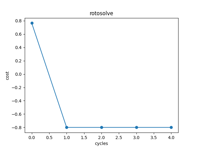
rotosolve¶

Rotosolve algorithm, which allows a direct jump to the optimal value of a single parameter relative to the fixed value of other parameters, can directly find the optimal parameters of the quantum circuit optimization algorithm.

class pyvqnet.optim.rotosolve.Rotosolve(max_iter=50)¶

Rotosolve: The rotosolve algorithm can be used to minimize a linear combination of quantum measurement expectation values. See the following paper: https://arxiv.org/abs/1903.12166, Ken M. Nakanishi. https://arxiv.org/abs/1905.09692, Mateusz Ostaszewski.

Parameters: max_iter – max number of iterations of the rotosolve update
Returns: a Rotosolve optimizer

Example:

from pyvqnet.optim.rotosolve import Rotosolve
import pyqpanda as pq
from pyvqnet.tensor import QTensor
from pyvqnet.qnn.measure import expval
machine = pq.CPUQVM()
machine.init_qvm()
nqbits = machine.qAlloc_many(2)

def gen(param,generators,qbits,circuit):
    if generators == "X":
        circuit.insert(pq.RX(qbits,param))
    elif generators =="Y":
        circuit.insert(pq.RY(qbits,param))
    else:
        circuit.insert(pq.RZ(qbits,param))
def circuits(params,generators,circuit):
    gen(params[0], generators[0], nqbits[0], circuit)
    gen(params[1], generators[1], nqbits[1], circuit)
    circuit.insert(pq.CNOT(nqbits[0], nqbits[1]))
    prog = pq.QProg()
    prog.insert(circuit)
    return prog

def ansatz1(params:QTensor,generators):
    circuit = pq.QCircuit()
    params = params.getdata()
    prog = circuits(params,generators,circuit)
    return expval(machine,prog,{"Z0":1},nqbits), expval(machine,prog,{"Y1":1},nqbits)

def ansatz2(params:QTensor,generators):
    circuit = pq.QCircuit()
    params = params.getdata()
    prog = circuits(params, generators, circuit)
    return expval(machine,prog,{"X0":1},nqbits)

def loss(params):
    Z, Y = ansatz1(params,["X","Y"])
    X = ansatz2(params,["X","Y"])
    return 0.5 * Y + 0.8 * Z - 0.2 * X

t = QTensor([0.3, 0.25])
opt = Rotosolve(max_iter=5)

costs_rotosolve = opt.minimize(t,loss)
print(costs_rotosolve)
# [0.7642691884821847, -0.799999999999997, -0.799999999999997, -0.799999999999997, -0.799999999999997]

Metrics¶

MSE¶

class pyvqnet.utils.metrics.MSE(y_true_Qtensor, y_pred_Qtensor)¶

MSE: Mean Squared Error.

Parameters

y_true_Qtensor – A QTensor of shape like (n_samples,) or (n_samples, n_outputs), true target value.
y_pred_Qtensor – A QTensor of shape like (n_samples,) or (n_samples, n_outputs), estimated target values.

Returns

return with float result.

Example:

import numpy as np
from pyvqnet.tensor import tensor
from pyvqnet.utils import metrics as vqnet_metrics
from pyvqnet import _core
_vqnet = _core.vqnet

y_true_Qtensor = tensor.arange(1, 12)
y_pred_Qtensor = tensor.arange(4, 15)
result = vqnet_metrics.MSE(y_true_Qtensor, y_pred_Qtensor)
print(result)
# 9.0

y_true_Qtensor = tensor.arange(1, 13).reshape([3, 4])
y_pred_Qtensor = tensor.arange(4, 16).reshape([3, 4])
result = vqnet_metrics.MSE(y_true_Qtensor, y_pred_Qtensor)
print(result)
# 9.0

RMSE¶

class pyvqnet.utils.metrics.RMSE(y_true_Qtensor, y_pred_Qtensor)¶

RMSE: Root Mean Squared Error.

Parameters

y_true_Qtensor – A QTensor of shape like (n_samples,) or (n_samples, n_outputs), true target value.
y_pred_Qtensor – A QTensor of shape like (n_samples,) or (n_samples, n_outputs), estimated target values.

Returns

return with float result.

Example:

import numpy as np
from pyvqnet.tensor import tensor
from pyvqnet.utils import metrics as vqnet_metrics
from pyvqnet import _core
_vqnet = _core.vqnet

y_true_Qtensor = tensor.arange(1, 12)
y_pred_Qtensor = tensor.arange(4, 15)
result = vqnet_metrics.RMSE(y_true_Qtensor, y_pred_Qtensor)
print(result)
# 3.0

y_true_Qtensor = tensor.arange(1, 13).reshape([3, 4])
y_pred_Qtensor = tensor.arange(4, 16).reshape([3, 4])
result = vqnet_metrics.RMSE(y_true_Qtensor, y_pred_Qtensor)
print(result)
# 3.0

MAE¶

class pyvqnet.utils.metrics.MAE(y_true_Qtensor, y_pred_Qtensor)¶

MAE: Mean Absolute Error.

Parameters

y_true_Qtensor – A QTensor of shape like (n_samples,) or (n_samples, n_outputs), true target value.
y_pred_Qtensor – A QTensor of shape like (n_samples,) or (n_samples, n_outputs), estimated target values.

Returns

return with float result.

Example:

import numpy as np
from pyvqnet.tensor import tensor
from pyvqnet.utils import metrics as vqnet_metrics
from pyvqnet import _core
_vqnet = _core.vqnet

y_true_Qtensor = tensor.arange(1, 12)
y_pred_Qtensor = tensor.arange(4, 15)
result = vqnet_metrics.MAE(y_true_Qtensor, y_pred_Qtensor)
print(result)
# 3.0

y_true_Qtensor = tensor.arange(1, 13).reshape([3, 4])
y_pred_Qtensor = tensor.arange(4, 16).reshape([3, 4])
result = vqnet_metrics.MAE(y_true_Qtensor, y_pred_Qtensor)
print(result)
# 3.0

R_Square¶

class pyvqnet.utils.metrics.R_Square(y_true_Qtensor, y_pred_Qtensor, sample_weight=None)¶

R_Square: R^2 (coefficient of determination) regression score function. The best possible score is 1.0, which can be negative (since the model can deteriorate arbitrarily). One that always predicts the expected value of y, ignoring the input features, will get an R^2 score of 0.0.

Parameters

y_true_Qtensor – A QTensor of shape like (n_samples,) or (n_samples, n_outputs), true target value.
y_pred_Qtensor – A QTensor of shape like (n_samples,) or (n_samples, n_outputs), estimated target values.
sample_weight – Array of shape like (n_samples,), optional sample weight, default:None.

Returns

return with float result.

Example:

import numpy as np
from pyvqnet.tensor import tensor
from pyvqnet.utils import metrics as vqnet_metrics
from pyvqnet import _core
_vqnet = _core.vqnet

y_true_Qtensor = tensor.arange(1, 12)
y_pred_Qtensor = tensor.arange(4, 15)
result = vqnet_metrics.R_Square(y_true_Qtensor, y_pred_Qtensor)
print(result)
# 0.09999999999999998

y_true_Qtensor = tensor.arange(1, 13).reshape([3, 4])
y_pred_Qtensor = tensor.arange(4, 16).reshape([3, 4])
result = vqnet_metrics.R_Square(y_true_Qtensor, y_pred_Qtensor)
print(result)
# 0.15625

precision_recall_f1_2_score¶

class pyvqnet.utils.metrics.precision_recall_f1_2_score(y_true_Qtensor, y_pred_Qtensor)¶

Calculate the precision, recall and F1 score of the predicted values under the 2-classification task. The predicted and true values need to be QTensors of similar shape (n_samples, ), with a value of 0 or 1, representing the labels of the two classes.

Parameters

y_true_Qtensor – A 1D QTensor, true target value.
y_pred_Qtensor – A 1D QTensor, estimated target value.

Returns

precision - precision result
recall - recall result
f1 - f1 score

Example:

import numpy as np
from pyvqnet.tensor import tensor
from pyvqnet.utils import metrics as vqnet_metrics
from pyvqnet import _core
_vqnet = _core.vqnet

y_true_Qtensor = tensor.QTensor([0, 0, 0, 0, 0, 1, 1, 1, 1, 1])
y_pred_Qtensor = tensor.QTensor([0, 0, 1, 1, 1, 0, 0, 1, 1, 1])

precision, recall, f1 = vqnet_metrics.precision_recall_f1_2_score(
    y_true_Qtensor, y_pred_Qtensor)
print(precision, recall, f1)
# 0.5 0.6 0.5454545454545454

precision_recall_f1_N_score¶

class pyvqnet.utils.metrics.precision_recall_f1_N_score(y_true_Qtensor, y_pred_Qtensor, N, average)¶

Precision, recall, and F1 score calculations for multi-classification tasks. where the predicted value and the true value are QTensors of similar shape (n_samples, ), and the values are integers from 0 to N-1, representing the labels of N classes.

Parameters

y_true_Qtensor – A 1D QTensor, true target value.
y_pred_Qtensor – A 1D QTensor, estimated target value.
N – N classes (number of classes).
average –
string, [‘micro’, ‘macro’, ‘weighted’]. This parameter is required for multi-class/multi-label targets.

'micro': Compute metrics globally by counting total true counts, false negatives and false positives.

'macro': Calculate the metric for each label and find its unweighted value. Meaning that the balance of labels is not considered.

'weighted': Calculate the metrics for each label and find their average (the number of true instances of each label). This changes 'macro' to account for label imbalance; this may result in F-scores not being between precision and recall.

Returns

precision - precision result
recall - recall result
f1 - f1 score

Example:

import numpy as np
from pyvqnet.tensor import tensor
from pyvqnet.utils import metrics as vqnet_metrics
from pyvqnet import _core
_vqnet = _core.vqnet

reference_list = [1, 1, 2, 2, 2, 3, 3, 3, 3, 3]
prediciton_list = [1, 2, 2, 2, 3, 1, 2, 3, 3, 3]
y_true_Qtensor = tensor.QTensor(reference_list)
y_pred_Qtensor = tensor.QTensor(prediciton_list)

precision_micro, recall_micro, f1_micro = vqnet_metrics.precision_recall_f1_N_score(
    y_true_Qtensor, y_pred_Qtensor, 3, average='micro')
print(precision_micro, recall_micro, f1_micro)
# 0.6 0.6 0.6

precision_macro, recall_macro, f1_macro = vqnet_metrics.precision_recall_f1_N_score(
    y_true_Qtensor, y_pred_Qtensor, 3, average='macro')
print(precision_macro, recall_macro, f1_macro)
# 0.5833333333333334 0.5888888888888889 0.5793650793650794

precision_weighted, recall_weighted, f1_weighted = vqnet_metrics.precision_recall_f1_N_score(
    y_true_Qtensor, y_pred_Qtensor, 3, average='weighted')
print(precision_weighted, recall_weighted, f1_weighted)
# 0.625 0.6 0.6047619047619047

precision_recall_f1_Multi_score¶

class pyvqnet.utils.metrics.precision_recall_f1_Multi_score(y_true_Qtensor, y_pred_Qtensor, N, average)¶

Precision, recall, and F1 score calculations for multi-classification tasks. where the predicted and true values are QTensors of similar shape (n_samples, N), where the values are N-dimensional one-hot encoded label values.

Parameters

y_true_Qtensor – A 1D QTensor, true target value.
y_pred_Qtensor – A 1D QTensor, estimated target value.
N – N classes (number of classes).
average –
string, [‘micro’, ‘macro’, ‘weighted’]. This parameter is required for multi-class/multi-label targets.

'micro': Compute metrics globally by counting total true counts, false negatives and false positives.

'macro': Calculate the metric for each label and find its unweighted value. Meaning that the balance of labels is not considered.

'weighted': Calculate the metrics for each label and find their average (the number of true instances of each label). This changes 'macro' to account for label imbalance; this may result in F-scores not being between precision and recall.

Returns

precision - precision result
recall - recall result
f1 - f1 score

Example:

import numpy as np
from pyvqnet.tensor import tensor
from pyvqnet.utils import metrics as vqnet_metrics
from pyvqnet import _core
_vqnet = _core.vqnet

reference_list = [[1, 0], [0, 1], [0, 0], [1, 1], [1, 0]]
prediciton_list = [[1, 0], [0, 0], [1, 0], [0, 0], [0, 0]]
y_true_Qtensor = tensor.QTensor(reference_list)
y_pred_Qtensor = tensor.QTensor(prediciton_list)

micro_precision, micro_recall, micro_f1 = vqnet_metrics.precision_recall_f1_Multi_score(y_true_Qtensor,
            y_pred_Qtensor, 2, average='micro')
print(micro_precision, micro_recall, micro_f1)
# 0.5 0.2 0.28571428571428575

macro_precision, macro_recall, macro_f1 = vqnet_metrics.precision_recall_f1_Multi_score(y_true_Qtensor,
            y_pred_Qtensor, 2, average='macro')
print(macro_precision, macro_recall, macro_f1)
# 0.25 0.16666666666666666 0.2

weighted_precision, weighted_recall, weighted_f1 = vqnet_metrics.precision_recall_f1_Multi_score(y_true_Qtensor,
            y_pred_Qtensor, 2, average='weighted')
print(weighted_precision, weighted_recall, weighted_f1)
# 0.3 0.19999999999999998 0.24

reference_list = [[1, 0, 0], [0, 1, 0], [0, 0, 1], [1, 1, 0], [1, 0, 1]]
prediciton_list = [[1, 0, 0], [1, 0, 0], [1, 1, 1], [1, 0, 0], [0, 1, 1]]
y_true_Qtensor = tensor.QTensor(reference_list)
y_pred_Qtensor = tensor.QTensor(prediciton_list)

micro_precision, micro_recall, micro_f1 = vqnet_metrics.precision_recall_f1_Multi_score(y_true_Qtensor,
            y_pred_Qtensor, 3, average='micro')
print(micro_precision, micro_recall, micro_f1) # 0.5 0.5714285714285714 0.5333333333333333

macro_precision, macro_recall, macro_f1 = vqnet_metrics.precision_recall_f1_Multi_score(y_true_Qtensor,
            y_pred_Qtensor, 3, average='macro')
print(macro_precision, macro_recall, macro_f1)
# 0.5 0.5555555555555555 0.5238095238095238

weighted_precision, weighted_recall, weighted_f1 = vqnet_metrics.precision_recall_f1_Multi_score(y_true_Qtensor,
            y_pred_Qtensor, 3, average='weighted')
print(weighted_precision, weighted_recall, weighted_f1)
# 0.5 0.5714285714285714 0.5306122448979592

auc_calculate¶

class pyvqnet.utils.metrics.auc_calculate(y_true_Qtensor, y_pred_Qtensor, pos_label=None, sample_weight=None, drop_intermediate=True)¶

Compute the precision, recall and f1 score of the classification task.

Parameters

y_true_Qtensor – A QTensor like of shape [n_samples]. A true binary label. If the label is not {1,1} or {0,1}, pos_label should be given explicitly.
y_pred_Qtensor – A QTensor like of shape [n_samples]. Target score, which can be a positive probability estimate class, confidence value, or a non-threshold measure of the decision (returned by “decision_function” on some classifiers)
pos_label – int or str. The label of the positive class. default=None. When pos_label is None, if y_true_Qtensor is at {-1,1} or {0,1}, pos_label is set to 1, otherwise an error will be raised.
sample_weight – array of shape (n_samples,), default=None.
drop_intermediate – boolean, optional (default=True). Whether to lower some suboptimal thresholds that don’t appear on the drawn ROC curve.

Returns

output float result.

Example:

import numpy as np
from pyvqnet.tensor import tensor
from pyvqnet.utils import metrics as vqnet_metrics
from pyvqnet import _core
_vqnet = _core.vqnet

y = np.array([1, 1, 1, 1, 0, 1, 0, 0, 0, 0])
pred = np.array([0.9, 0.8, 0.7, 0.6, 0.6, 0.4, 0.4, 0.3, 0.2, 0.1])
y_Qtensor = tensor.QTensor(y)
pred_Qtensor = tensor.QTensor(pred)
result = vqnet_metrics.auc_calculate(y_Qtensor, pred_Qtensor)
print("auc:", result)
# 0.92

y = np.array([1, 1, 1, 1, 1, 0, 0, 1, 1, 1])
pred = np.array([1, 0, 1, 1, 1, 1, 0, 1, 1, 0])
y_Qtensor = tensor.QTensor(y)
pred_Qtensor = tensor.QTensor(pred)
result = vqnet_metrics.auc_calculate(y_Qtensor, pred_Qtensor)
print("auc:", result)
# 0.625

y = [1, 2, 1, 1, 1, 0, 0, 1, 1, 1]
pred = [1, 0, 2, 1, 1, 1, 0, 1, 1, 0]
y_Qtensor = tensor.QTensor(y)
pred_Qtensor = tensor.QTensor(pred)
result = vqnet_metrics.auc_calculate(y_Qtensor, pred_Qtensor, pos_label=2)
print("auc:", result)
# 0.1111111111111111